As computing power grows, materials science researchers are developing higher fidelity models to capture smaller length and briefer time scales — where the action takes place — of materials under stress. 

Ultimate accuracy in modeling at the atomic level comes from quantum chemistry calculations such as density functional theory (DFT), which solve Schrödinger’s equation and simulate interactions between electrons. However, these methods don’t scale well with large number of atoms; quantum system sizes are typically limited to less than a thousand atoms. 

Instead, a preferred method called molecular dynamics (MD) uses Newton’s equations of motion to describe atom behavior. MD tracks the motion of billions of atoms by repeatedly calculating the atomic forces over very many, exceedingly tiny, intervals of time. MD is much faster and scales better than DFT, but it does not explicitly include electrons, a weakness. Instead, MD typically uses simple empirical models to relate atom positions to forces. The model parameters can be adjusted to approximately mimic specific materials, but these models can not accurately match DFT results in detail.

Machine learning to the rescue 

Recently, however, empirical models are being replaced with machine learning methods, which can approach DFT accuracy at a fraction of the cost, and also scale much better than DFT with respect to the number of atoms included in the target sample. MD simulations then can bridge the gap between expensive quantum chemistry calculations and lower fidelity continuum methods that omit atomic level details. (Continuum methods resolve the behavior of 3D “chunks” of continuous material, while MD resolves the motion of individual atoms.) 

MD length scales are still extremely small compared to a grain of sand or a glass of water, and time scales are similarly small. However, with state-of-the-art computing power, MD simulations of billions to trillions of atoms can approach the length and time scales necessary for real-world experiments in some cases. Additionally, information from MD simulations can be used improve continuum methods in a multi-scale workflow. 

Better understanding of the kinetics of the liquid to vapor phase transition is essential in building models that more accurately represent what is happening and thereby reduce the difference between code prediction and experimental measurement. 

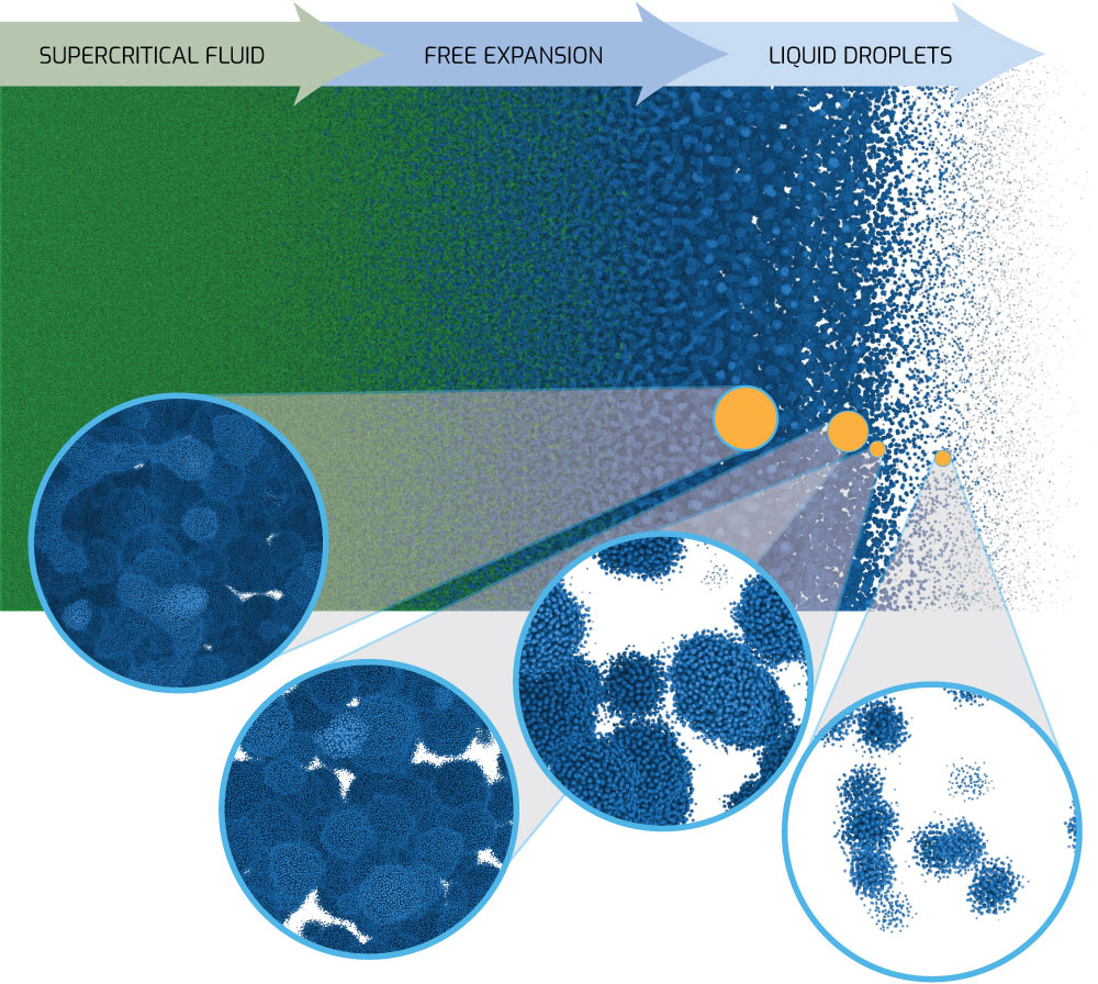
One such application is the free expansion of molten metal, for example when an electrical pulse rapidly heats and melts a thin wire up to a supercritical temperature. Supercritical means the molten metal is so hot that there is no longer a clear distinction between the liquid and vapor phases. However, when the supercritical fluid expands, the temperature drops below the critical temperature, where the fluid rapidly separates into liquid droplets and vapor bubbles. 

Bridging practice and theory of free expansion at Sandia’s Z machine

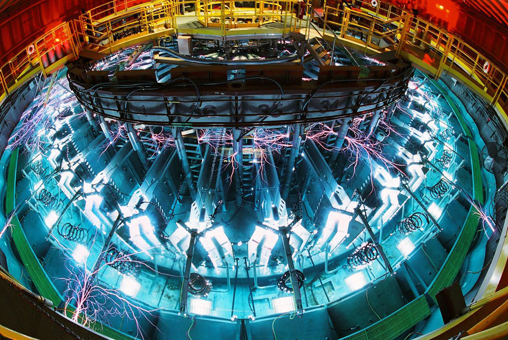
For some flyers and wire vaporization experiments on Sandia’s Z machine, as well as other platforms, the expanding material enters this mixed phase (liquid/vapor) regime.  Continuum simulation codes generally assume an equilibrium material approximation in the mixed phase and apply some type of averaging to account for how much vapor vs. liquid is present. 

For a system in equilibrium, this is a valid approximation. However, a rapidly expanding material is not in equilibrium. When the leading edge of the expanding material reaches a low enough density below the critical temperature, it should transform from a liquid to a vapor at a material dependent kinetic rate, or even experience spinodal (spontaneous) decomposition. The material further inside will continue to expand based on how much back pressure is at and near the leading edge, and such information will continue to propagate through the rarefaction wave. 

If the transformation rate from liquid to vapor is wrong due to incorrect kinetics approximations, then the expansion velocity that simulations predict will also be wrong after some time. This information propagates through the material until, in the case of flyers on the Z machine or Thor, the measured velocity at the front of a flyer and the simulated flyer velocity will diverge. Similar effects would occur on other platforms and has caused severe problems in wire initiation simulations where the energy to vaporize thicker wires is predicted to be less than seen in Z experiments. New computational work using MD is intended to lessen this disparity. 

Researchers at Sandia started out using an efficient, empirical potential called the Lennard-Jones (LJ) model to examine free expansion with MD. One of LJ’s nice features is that it can be written as a single equation with only two free parameters. Even though it is simple, the LJ model captures many relevant physics phenomena such as the transition from supercritical fluid to subcritical phase separation into liquid and vapor phases seen in free expansion. Huge (multi-billion atom) LJ simulations have been run on the Lawrence Livermore National Laboratory Sierra supercomputer to investigate the physics of free expansion. 

The key advantage of MD in this case is that it avoids making any explicit assumptions about the material behavior (droplet formation, coalescence, break-up, surface tension, heat transfer) commonly needed for continuum models. Researchers are now transitioning to a more realistic — but computationally expensive — model for aluminum metal using the SNAP (Spectral Neighbor Analysis Potential) machine-learning method fit to DFT data. SNAP, developed at Sandia, can be used to scale up models to much larger length and time scales than DFT while preserving high accuracy. Thus, SNAP atomistic simulations will offer unprecedented insight into phase change kinetics and fluid microstructure evolution directly relevant to experimental studies of free expansion.